Excel PIVOTBY: Build Pivot-Style Summaries With a Formula

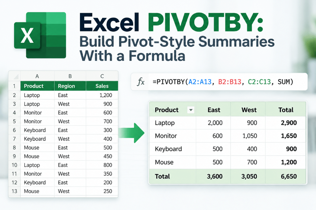
The Excel PIVOTBY function can create a two-dimensional summary using a normal formula.

You can group information by rows and columns, calculate totals with SUM, AVERAGE, COUNT, and other functions, and have the result update dynamically when the source data changes.

What Does Excel PIVOTBY Do?

PIVOTBY groups data across two dimensions and summarizes the associated values.

Its basic syntax is:

=PIVOTBY(row_fields,col_fields,values,function)

The four main arguments are:

row_fields – What should appear down the rows.

col_fields – What should appear across the columns.

values – The numbers you want to summarize.

function – How Excel should summarize them, such as SUM, AVERAGE, or COUNT.

A Simple PIVOTBY Example

Imagine your worksheet contains:

Year in column A
Region in column B
Sales in column C

You could use:

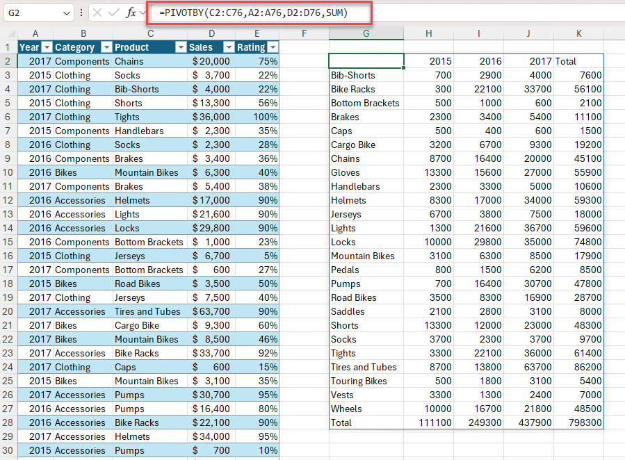
=PIVOTBY(B2:B100,A2:A100,C2:C100,SUM)

Excel can create a summary showing:

Region	2024	2025	2026
North	Total	Total	Total
South	Total	Total	Total
West	Total	Total	Total

The rows are grouped by Region.

The columns are grouped by Year.

Sales are added together using SUM.

Microsoft uses the same general type of example to demonstrate summarizing sales by two categories.

PIVOTBY Is Similar to a PivotTable – But Not the Same

PIVOTBY can produce a result that looks very similar to a traditional PivotTable.

However, Microsoft specifically notes that PIVOTBY is not directly related to Excel’s PivotTable feature.

The biggest practical difference is how you create the result.

A PivotTable is created through Excel’s PivotTable interface.

PIVOTBY is simply a formula entered into a cell.

That means the result can fit naturally into worksheets that already rely heavily on formulas and dynamic arrays.

Use AVERAGE Instead of SUM

You are not limited to adding values together.

For example:

=PIVOTBY(B2:B100,A2:A100,C2:C100,AVERAGE)

returns the average value for each combination of Region and Year.

You can also use aggregation functions such as:

SUM
AVERAGE
COUNT
MAX
MIN

Microsoft also allows supported LAMBDA-based aggregation functions for more advanced calculations.

Can PIVOTBY Add Totals?

Yes.

PIVOTBY includes optional arguments that control grand totals and subtotals.

For example, you can choose to display:

No totals
Grand totals
Grand totals and subtotals
Totals at the top instead of the bottom

Microsoft’s row_total_depth and col_total_depth arguments control how totals appear in the result.

For basic summaries, however, you can often leave these optional arguments out and let Excel handle them automatically.

Can You Sort PIVOTBY Results?

Yes.

PIVOTBY includes separate sorting options for its row and column fields.

This means you can create a summary and control the order directly from the formula.

For example, Microsoft’s documentation demonstrates a PIVOTBY formula that sorts summarized sales in descending order.

This can be useful for reports where you want the highest-performing categories to appear first.

Filter the Data Before Summarizing It

PIVOTBY also includes an optional filter_array argument.

That means you can exclude rows that do not meet a condition before Excel creates the summary.

For example, you could build a report that only includes:

One department
Active products
Sales above a certain amount
Transactions from a specific period

This gives PIVOTBY some of the filtering flexibility normally associated with more complex report formulas.

PIVOTBY vs GROUPBY

Excel also has a related function called GROUPBY.

The main difference is the number of dimensions.

GROUPBY groups data along one axis.

PIVOTBY groups data along two axes.

For example:

GROUPBY(Region,Sales,SUM)

might give you total sales by Region.

PIVOTBY could instead give you:

Region × Year

with sales summarized inside the table.

So if you need a simple one-direction summary, GROUPBY may be enough.

If you need both row and column categories, PIVOTBY is the better fit.

PIVOTBY vs PivotTable

Use PIVOTBY when:

You prefer formulas
You want a dynamic-array result
You want the summary embedded in another formula-based report
You need automatic recalculation
You want grouping across rows and columns

Use a traditional PivotTable when:

You prefer drag-and-drop controls
You want interactive field rearranging
You need PivotTable-specific tools
Other users need to explore the data manually

Neither option completely replaces the other.

Which Excel Versions Support PIVOTBY?

Microsoft’s current documentation is slightly inconsistent here.

The dedicated PIVOTBY support page lists Microsoft 365 as well as several perpetual Excel releases, while Microsoft’s alphabetical function directory currently labels PIVOTBY as a Microsoft 365 function.

If Excel returns:

#NAME?

when you enter PIVOTBY, your installed Excel version or build may not currently support the function.

Final Thoughts

Excel PIVOTBY brings PivotTable-style summarizing into a normal Excel formula.

With something as simple as: