How to Create Pivot Tables in Excel

PivotTables are one of the most useful tools in Excel for summarizing and analyzing data. Microsoft says a PivotTable helps you calculate, summarize, and analyze data so you can see comparisons, patterns, and trends more clearly.

They are especially useful when you have a large table and want quick answers like totals by category, counts by name, or averages by month without writing complicated formulas. Microsoft’s support page for PivotTables in Excel for Windows says the basic setup starts by selecting your data, choosing Insert > PivotTable, then deciding where the PivotTable should appear.

The Short Answer

To create Pivot Tables in Excel:

select the data you want to analyze
go to Insert
click PivotTable
choose where the PivotTable should go
click OK
drag fields into Rows, Columns, Values, and Filters

Microsoft says this is the normal workflow for creating a PivotTable from an existing table or range in Excel for Windows.

What You Need Before Creating a PivotTable

Before you build a PivotTable, your source data should be organized properly.

Microsoft says your data should be organized in columns with a single header row. That setup helps Excel understand the field names and structure correctly when generating the PivotTable.

A good PivotTable source usually has

one row of column headers
no empty header cells
consistent data under each column
one row per record or entry

If the source data is messy, the PivotTable can still be created, but the results are usually harder to read and manage. That follows from Microsoft’s note about organizing data in columns with a single header row.

How to Create a PivotTable in Excel

This is the standard method most users will use.

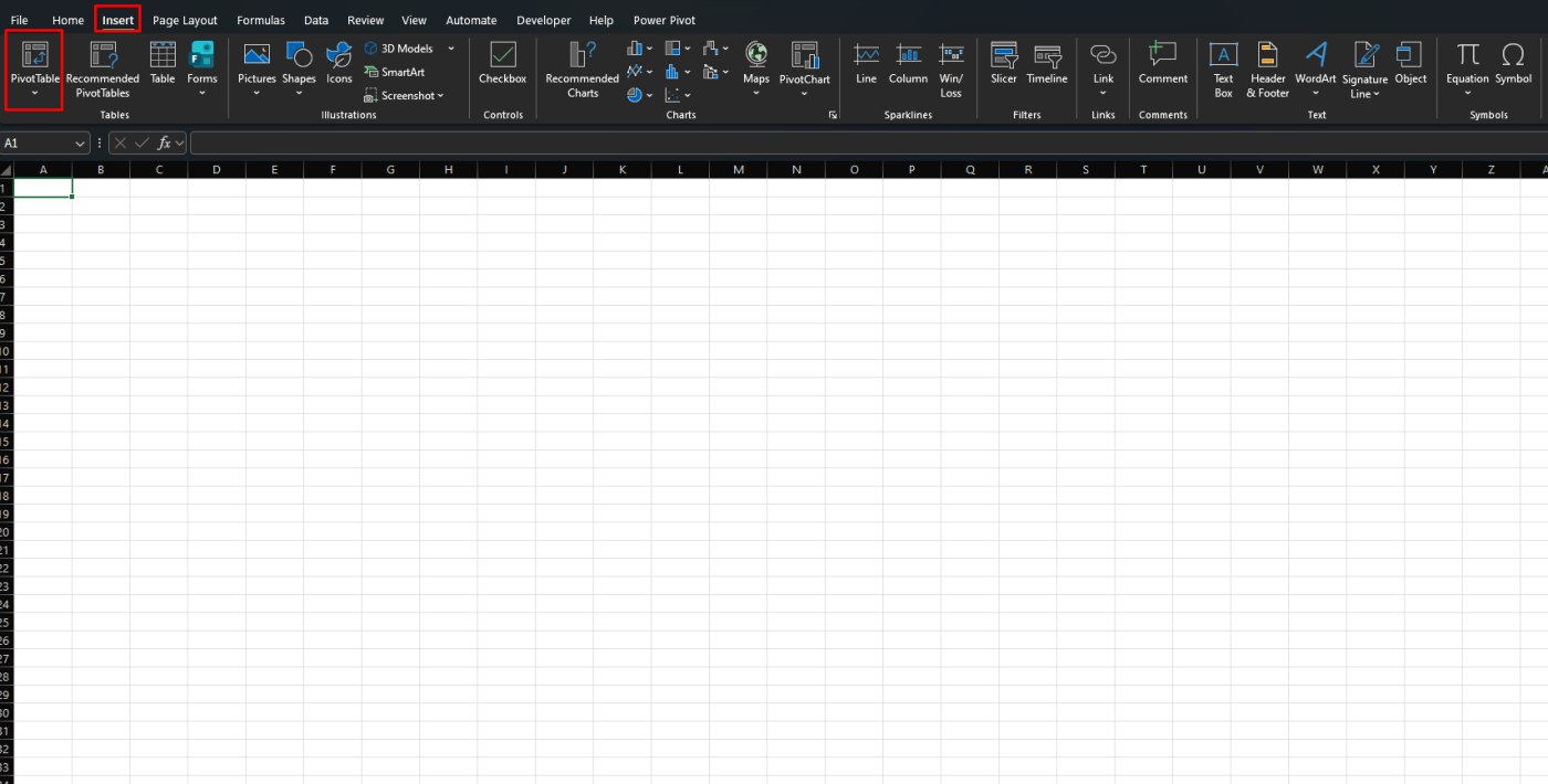
Microsoft says to select the cells you want to use, then choose Insert > PivotTable. Excel creates the PivotTable from the selected table or range and then asks where you want the report placed.

Step-by-step

select the cells you want to use
go to Insert > PivotTable
choose New Worksheet or Existing Worksheet
click OK

Microsoft says New Worksheet places the PivotTable on a new sheet, while Existing Worksheet lets you choose a location in the current workbook.

How PivotTable Fields Work

Once the PivotTable is created, Excel gives you fields to arrange.

The basic idea is simple:

Rows show categories vertically
Columns show categories across the top
Values contain the numbers being summarized
Filters let you narrow the report

Microsoft’s support area for PivotTables links directly to its Field List guidance, which is where these layout choices are arranged in practice.

Simple PivotTable Example

Imagine you have a sales table with these columns:

Salesperson
Region
Product
Amount

You could build a PivotTable like this:

drag Region to Rows
drag Amount to Values

Excel will then summarize the sales amount by region. This is the kind of comparison and summary Microsoft says PivotTables are designed to help with.

You could also:

drag Salesperson to Rows
drag Amount to Values

That would show totals by salesperson instead.

How to Change What the PivotTable Calculates

By default, Excel often sums numeric values, but that is not your only option.

PivotTables are commonly used for:

Sum
Count
Average
Max
Min

Microsoft describes PivotTables as tools to calculate and summarize data, which is why changing the value summary type is such a core part of using them.

This is useful when:

you want totals instead of counts
you want averages instead of sums
you want the number of entries in each category

How to Filter a PivotTable

Filters make PivotTables much more useful.

You can place a field into the Filters area to narrow the results. For example:

put Region in Filters
view only one region at a time

Microsoft’s PivotTable support pages also connect PivotTables with tools like slicers and filtering, which shows that narrowing what you see is a major part of how PivotTables are used.

How to Create a PivotTable in a New Worksheet

For most people, this is the cleanest option.

Microsoft says when you create a PivotTable, you can select New Worksheet so Excel places it on a separate sheet. That keeps the report away from the raw data and usually makes the workbook easier to manage.

This is usually best when:

your source data is large
you want a cleaner workbook
you plan to build more than one PivotTable

How to Create a PivotTable in the Same Worksheet

Microsoft also says you can choose Existing Worksheet and then select where the PivotTable should appear.

This can be useful if:

you want the summary close to the source data
the workbook is small
you are building a compact report

Other PivotTable Sources in Excel

The normal source is a table or range, but Microsoft says the PivotTable dropdown also offers other possible sources. In addition to an existing table or range, Microsoft lists options such as an external data source and the workbook’s Data Model.

That matters more for advanced users, but it is useful to know PivotTables are not limited to one simple worksheet range.

FAQ

How do I create a PivotTable in Excel?

Microsoft says to select the cells you want to use, then choose Insert > PivotTable, decide where the report should be placed, and click OK.

What kind of data works best for a PivotTable?

Microsoft says your data should be organized in columns with a single header row.

Should I place a PivotTable in a new worksheet?

Microsoft says you can choose either New Worksheet or Existing Worksheet. New Worksheet is often cleaner because it keeps the report separate from the raw data.