Instructions
How to Use VLOOKUP in Excel
May
VLOOKUP is one of the most widely used Excel functions for finding data in a table. Microsoft says you use VLOOKUP when you need to find things in a table or range by row, such as looking up a price by part number or finding an employee name from an ID.
VLOOKUP is useful because it searches the first column of a selected range and returns a value from another column in the same row. Microsoft also notes one of the biggest limits of VLOOKUP: the value you want to look up must be in the first column of the table array, with the return value somewhere to the right.
The Short Answer
The basic VLOOKUP formula is:
=VLOOKUP(lookup_value, table_array, col_index_num, [range_lookup])
Microsoft says:
- lookup_value is the value you want to find
- table_array is the range where Excel searches
- col_index_num is the number of the column that contains the return value
- range_lookup controls whether the match is approximate or exact
In most everyday cases, you will use FALSE for an exact match.
How VLOOKUP Works
Microsoft says VLOOKUP searches for a value in the first column of a range and returns a value from another column in the same row.
That means VLOOKUP works best when:
- your lookup value is on the left
- the result you want is in a column to the right
- your table is structured clearly
If the value you want to return is to the left of the lookup column, VLOOKUP is not the best tool. Microsoft’s lookup reference suggests XLOOKUP as a newer function that works in any direction and returns exact matches by default.
Basic VLOOKUP Example
Imagine:
- column A has product IDs
- column B has product names
- cell E2 contains the ID you want to search for
Your formula could be:
=VLOOKUP(E2,A2:B20,2,FALSE)
This tells Excel to:
- look for the value in E2
- search in the range A2:B20
- return the value from the second column
- use FALSE for an exact match
Microsoft’s VLOOKUP guide gives this same style of exact-match example and explains that FALSE returns an exact match.
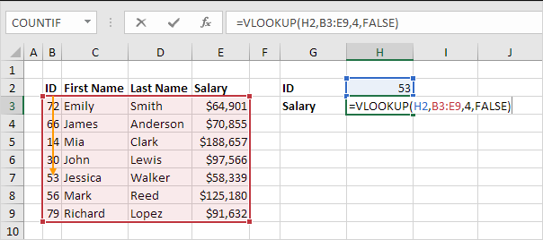
How to Use Exact Match in VLOOKUP
For most users, exact match is the safest option.
Microsoft says 0/FALSE means exact match, while 1/TRUE means approximate match.
Example:
=VLOOKUP(E2,A2:B20,2,FALSE)
Use this when:
- looking up IDs
- matching product codes
- finding exact names
- searching unsorted lists
This is the version most beginners should use first.
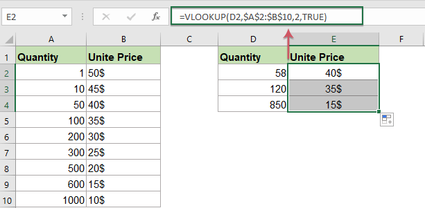
How to Use Approximate Match in VLOOKUP
Approximate match is useful, but only in specific situations.
Microsoft says 1/TRUE means approximate match, and it also warns that for approximate matching, the first column of the table should be sorted in ascending order. Otherwise, the result may be incorrect.
Example:
=VLOOKUP(E2,A2:B20,2,TRUE)
This is useful for:
- grade bands
- discount levels
- tax brackets
- score categories
If the first column is not sorted properly, approximate match can return the wrong result.
What Each Part of VLOOKUP Means
Microsoft breaks the formula into four parts.
lookup_value
This is the value you want to find. Microsoft says it can be a typed value or a cell reference.
table_array
This is the full range Excel searches in. Microsoft says the first column in this range must contain the lookup value.
col_index_num
This is the column number in the selected range that contains the return value. Microsoft says numbering starts at 1 for the left-most column of the table array.
range_lookup
This controls match type:
- FALSE = exact match
- TRUE = approximate match
Common VLOOKUP Mistakes to Avoid
The lookup value is not in the first column
Microsoft says the value you want to look up must be in the first column of the table array. If it is not, VLOOKUP will not work the way you expect.
Using the wrong column number
If your col_index_num points to the wrong column, Excel will return the wrong result even if the lookup itself works.
Using TRUE on unsorted data
Microsoft says approximate match requires the first column to be sorted in ascending order. If it is not sorted, the result can be incorrect.
Storing numbers or dates as text
Microsoft’s best-practices section warns not to store number or date values as text in the lookup column, because VLOOKUP may return incorrect or unexpected results.
When to Use VLOOKUP vs XLOOKUP
VLOOKUP still works well, but Microsoft’s lookup reference now points users toward XLOOKUP as the newer option.
Microsoft says XLOOKUP is an improved version of VLOOKUP that works in any direction and returns exact matches by default.
That means:
- use VLOOKUP if you are working with older Excel versions or classic tables
- use XLOOKUP if you want more flexibility in newer Excel versions
Best Use Cases for VLOOKUP
VLOOKUP is especially useful for:
- product tables
- employee lists
- price lookups
- inventory sheets
- student records
- basic lookup tasks in older workbooks
It is one of the easiest lookup functions to learn when your table is arranged in the standard left-to-right way.
FAQ
What is VLOOKUP in Excel?
Microsoft says VLOOKUP is used to find things in a table or range by row, such as a price by part number or an employee name by ID.
What is the syntax of VLOOKUP?
Microsoft says the syntax is:
=VLOOKUP(lookup_value, table_array, col_index_num, [range_lookup])
Should I use TRUE or FALSE in VLOOKUP?
Microsoft says FALSE is for exact match and TRUE is for approximate match. For most everyday lookups, exact match is the safer option.
Why is VLOOKUP not working correctly?
Common reasons include the lookup value not being in the first column, the wrong column index number, unsorted data with approximate match, or numbers and dates stored as text. Microsoft’s best-practices section warns about all of these.
Get more done with genuine Office keys, fast delivery, and simple activation that keeps your Excel tools ready from the start.