Excel FILTER Function: Create Lists That Update Automatically

Need a list in Excel that automatically changes when your source data changes?

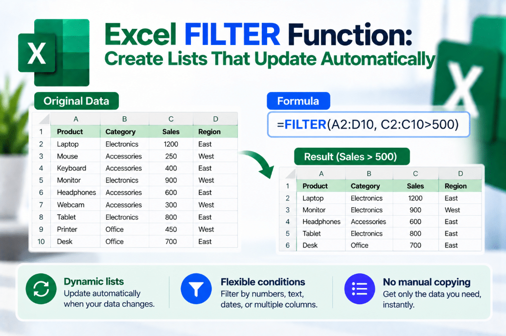
The Excel FILTER function can return only the rows that match your conditions and update the result automatically.

Unlike the normal Filter button, FILTER creates a separate dynamic list instead of hiding rows in your original table.

What Does the Excel FILTER Function Do?

FILTER returns data from a range based on a condition you define.

Its syntax is:

=FILTER(array,include,[if_empty])

The arguments are:

array – The range you want returned.

include – The condition that decides which rows or columns should appear.

if_empty – Optional result to display if nothing matches.

Microsoft describes FILTER as filtering an array using a TRUE/FALSE condition array.

A Simple FILTER Example

Suppose A2 contains:

• Product
• Category
• Price

If column B contains the category and you only want products marked Laptop, use:

=FILTER(A2:C20,B2:B20="Laptop")

Excel returns every matching row.

If you add another Laptop to the source range, the filtered result updates automatically.

Filter Using a Cell Value

You do not need to type the condition directly into the formula.

For example, if E2 contains:

Laptop

you can use:

=FILTER(A2:C20,B2:B20=E2)

Now you can change E2 to:

Monitor

and the result updates to show only monitors.

This is useful for dashboards and interactive reports where users choose a category from another cell.

What Happens If Nothing Matches?

If no rows meet your condition, FILTER can return a calculation error unless you use the optional third argument.

For example:

=FILTER(A2:C20,B2:B20=E2,"No results")

If nothing matches, Excel displays:

No results

You can also return a blank:

=FILTER(A2:C20,B2:B20=E2,"")

Microsoft includes the if_empty argument specifically for this situation.

Filter Numbers Greater Than a Value

FILTER is not limited to text.

Suppose column C contains prices.

To return products costing more than 100:

=FILTER(A2:C20,C2:C20>100)

You can also reference another cell:

=FILTER(A2:C20,C2:C20>F2)

Now the minimum price is controlled by the value entered in F2.

Use Multiple Conditions With AND

You can filter using more than one condition.

Suppose you want:

• Category = Laptop
• Price less than 1000

Use:

=FILTER(A2:C100,(B2:B100="Laptop")*(C2:C100<1000),"No results")

The multiplication symbol * works like AND.

Both conditions must be TRUE for a row to appear.

Microsoft uses this same technique in its FILTER examples for combining multiple conditions.

Use Multiple Conditions With OR

You can also return rows where either condition is true.

For example:

=FILTER(A2:C100,(B2:B100="Laptop")+(B2:B100="Monitor"),"No results")

The plus symbol + works like OR.

This returns rows where the category is either Laptop or Monitor.

Combine FILTER With SORT

FILTER becomes even more useful when combined with other dynamic-array functions.

For example:

=SORT(FILTER(A2:C100,B2:B100="Laptop"),3,-1)

This formula:

1. Filters the table to show only laptops
2. Sorts the result by column 3
3. Displays the highest values first

Microsoft also documents combining FILTER and SORT to create filtered and automatically sorted results.

FILTER vs the Normal Excel Filter

The normal Data → Filter feature temporarily hides rows that do not match your criteria.

The FILTER function works differently.

It creates a completely separate result in another part of the worksheet.

That makes FILTER especially useful when you want to:

• Build dashboards
• Create automatic reports
• Display category-specific lists
• Create search-style results
• Keep the original table unchanged
• Combine filtering with other formulas

Traditional AutoFilter is still useful when you simply want to temporarily hide data inside an existing table.

Why Does FILTER Spill Into Other Cells?

FILTER is a dynamic-array function.

The formula only needs to be entered in one cell, and Excel automatically fills the surrounding cells with all matching results.

You do not need to copy the formula down manually.

If something blocks the output area, Excel may display a #SPILL! error.

Make sure the cells where the result needs to appear are empty.

FILTER With UNIQUE

Another useful combination is FILTER with UNIQUE.

For example:

=UNIQUE(FILTER(B2:B100,A2:A100="North"))

This can return a list of unique values only for records that meet a particular condition.

You can then use the result for reports, dropdown lists, or summaries.

Which Excel Versions Support FILTER?

Microsoft currently lists FILTER for:

• Excel for Microsoft 365
• Excel for Microsoft 365 for Mac
• Excel 2024
• Excel 2024 for Mac
• Excel 2021
• Excel 2021 for Mac
• Supported Excel mobile apps

Microsoft’s function directory marks FILTER as an Excel 2021 function, meaning it is not limited to Microsoft 365 or Excel 2024.

Final Thoughts

The Excel FILTER function is one of the easiest ways to create lists that update automatically.

Instead of manually filtering and copying data, you can define a condition once and let Excel continuously return the matching records.

You can also combine FILTER with SORT, UNIQUE, and other dynamic-array functions to build powerful reports from a single formula.

Need Microsoft Office with modern Excel functions? Explore our Microsoft Office keys and choose the version that fits your work today.