Excel WRAPROWS: Turn One Long List Into a Table

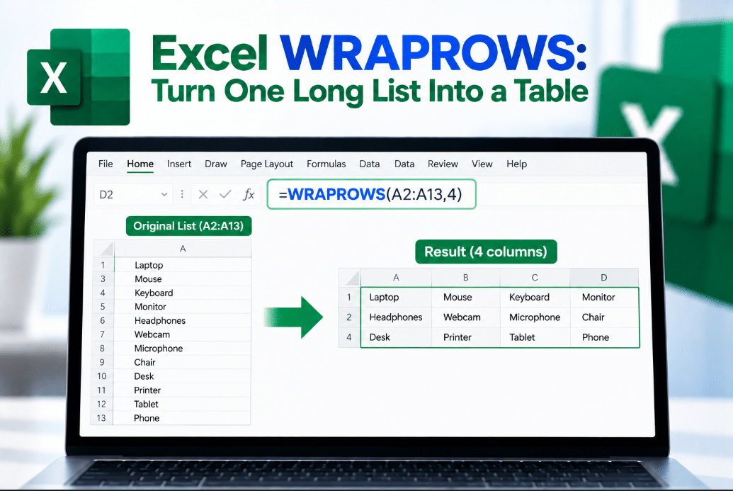
Have a long list of values that would look much better arranged across several rows and columns?

The Excel WRAPROWS function can reshape that list automatically.

Instead of manually copying values into a table, you tell Excel how many items should appear in each row, and WRAPROWS creates the new layout for you.

What Does Excel WRAPROWS Do?

WRAPROWS takes a one-dimensional row or column and turns it into a two-dimensional array.

Its syntax is:

=WRAPROWS(vector,wrap_count,[pad_with])

The arguments mean:

vector – The original row or column you want to reshape.

wrap_count – The maximum number of values you want in each row.

pad_with – Optional value Excel should use if the final row does not contain enough items.

Microsoft explains that WRAPROWS fills the new array row by row until all source values have been used.

A Simple WRAPROWS Example

Suppose A1 contains the numbers 1 through 12.

Enter:

=WRAPROWS(A1:A12,4)

Excel returns:

1 2 3 4
5 6 7 8
9 10 11 12

The 4 tells Excel to place four values in each row.

The formula automatically spills into the required cells.

Turn One Long List Into Three Columns

Imagine you have a long list of product names in A2.

If you want three products per row, use:

=WRAPROWS(A2:A100,3)

Excel creates a table with three columns and as many rows as needed.

This can be useful for:

• Product lists
• Name lists
• Labels
• Codes
• Inventory layouts
• Dashboard displays
• Printing compact lists

You do not need to manually calculate where each item belongs.

What Does Wrap Count Mean?

The wrap_count controls how many values appear before Excel starts a new row.

For example:

=WRAPROWS(A1:A20,5)

creates rows containing up to five values each.

Using:

=WRAPROWS(A1:A20,2)

creates rows containing only two values.

A larger wrap count creates a wider table.

A smaller wrap count creates a taller table.

What Happens If the Last Row Is Not Full?

Suppose your list contains 10 values and you use:

=WRAPROWS(A1:A10,4)

Excel needs three rows:

• First row: 4 values
• Second row: 4 values
• Third row: 2 values

By default, the remaining spaces in the last row display #N/A.

You can change this with the optional pad_with argument.

For example:

=WRAPROWS(A1:A10,4,"")

uses blank cells instead.

This often gives the result a cleaner appearance.

Use Your Own Fill Value

The padding does not have to be blank.

For example:

=WRAPROWS(A1:A10,4,"N/A")

fills unused cells with the text:

N/A

You could also use:

=WRAPROWS(A1:A10,4,"-")

to display a dash.

Microsoft specifically supports this optional padding argument for incomplete rows.

Can WRAPROWS Start With a Horizontal List?

Yes.

Your source does not have to be a vertical column.

For example, if A1 contains a horizontal list:

=WRAPROWS(A1:J1,3)

Excel can still reshape those values into several rows.

The source simply needs to be a one-dimensional array, meaning one row or one column.

Why Does WRAPROWS Show #VALUE!?

WRAPROWS expects a one-dimensional source.

If you give it a range containing several rows and several columns, Excel can return #VALUE!.

For example, this may cause a problem:

=WRAPROWS(A1:C10,3)

because A1 is already a two-dimensional range.

Microsoft states that WRAPROWS returns #VALUE! when the supplied vector is not one-dimensional.

Why Does WRAPROWS Show #NUM!?

The wrap count must be at least 1.

For example:

=WRAPROWS(A1:A10,0)

returns #NUM! because Excel cannot create rows containing zero values.

Use 1 or a larger number instead.

WRAPROWS vs WRAPCOLS

Excel also includes a related function called WRAPCOLS.

The difference is simple:

WRAPROWS fills the new array across rows.

WRAPCOLS fills the new array down columns.

For example, WRAPROWS with a wrap count of 3 places three items across each row.

WRAPCOLS with a wrap count of 3 places three items down each column.

Which one you use depends on the layout you want.

Which Excel Versions Support WRAPROWS?

Microsoft currently lists WRAPROWS for:

• Excel for Microsoft 365
• Excel for Microsoft 365 for Mac
• Excel 2024
• Excel 2024 for Mac

Microsoft’s function list also identifies WRAPROWS as an Excel 2024 function.

If Excel displays #NAME? when you enter WRAPROWS, your Excel version may not support it.

Final Thoughts

Excel WRAPROWS is a simple way to turn one long row or column into a more compact table.

For example:

=WRAPROWS(A1:A100,5)

automatically arranges the list into rows containing five values each.

You can also control what appears in unused cells and change the wrap count whenever you want a different layout.

For product lists, labels, codes, dashboards, and other long datasets, WRAPROWS can save a lot of manual copying and rearranging.

Need Microsoft Office with modern Excel functions? Explore our Microsoft Office keys and choose the version that fits your work today.