Instructions
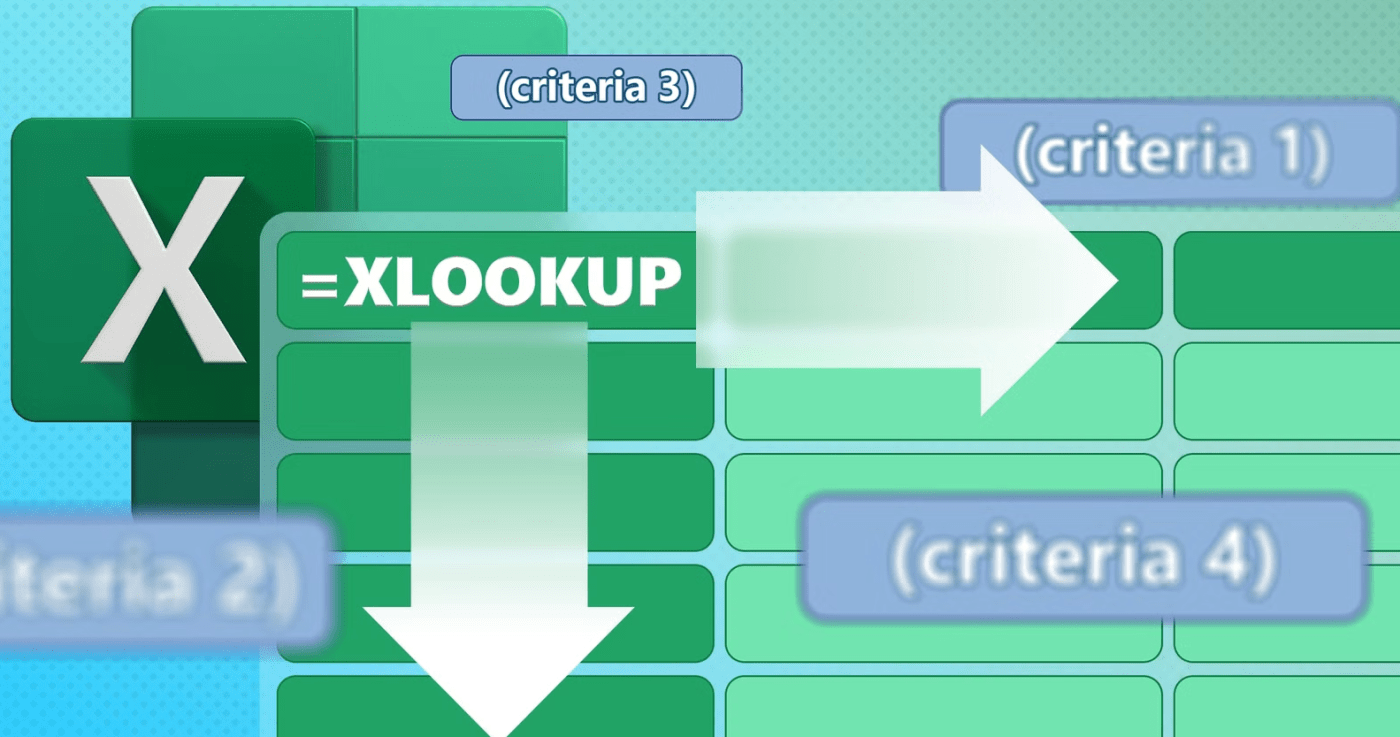
How to Use XLOOKUP in Excel
May
XLOOKUP is one of the most useful modern Excel functions because it helps you find a value in one column and return a matching result from another column. Microsoft says you can use XLOOKUP to look up things in a table or range by row, such as finding a part price by part number or finding an employee name from an ID. Microsoft also notes that XLOOKUP can return a result from another column regardless of whether that return column is to the left or right of the lookup column.
For many users, XLOOKUP is easier and more flexible than older lookup methods because it supports exact matching by default, lets you define what happens if no result is found, and can also search from the end of a list when needed. Microsoft’s official function page describes all of these options in the XLOOKUP syntax.
The Short Answer
To use XLOOKUP in Excel, the basic formula is:
=XLOOKUP(lookup_value, lookup_array, return_array)
Microsoft says the full syntax is:
=XLOOKUP(lookup_value, lookup_array, return_array, [if_not_found], [match_mode], [search_mode])
In that syntax, lookup_value is what you want to find, lookup_array is where Excel searches, and return_array is the range Excel returns the answer from.
How XLOOKUP Works
Microsoft says XLOOKUP searches a range or array and returns the item that matches the first result it finds. If no match exists, it can also return the closest approximate match, depending on the options you choose.
The three required parts
These are the main parts of XLOOKUP:
- lookup_value = the value you want to search for
- lookup_array = the column or row where Excel searches
- return_array = the column or row that contains the answer you want returned
Microsoft lists those three as the required core arguments in the function syntax.
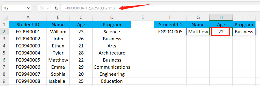
Basic XLOOKUP Example
This is the most common way people use it.
Imagine:
- column A contains product IDs
- column B contains product names
- cell E2 contains the product ID you want to search for
Your formula could be:
=XLOOKUP(E2,A2:A20,B2:B20)
Microsoft says XLOOKUP can look in one column for a search term and return a result from the same row in another column. That is exactly what this example does.
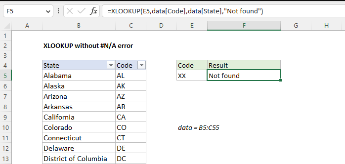
How to Show a Custom Result If Nothing Is Found
One of the best XLOOKUP features is that you can control what happens when there is no match.
Microsoft says the optional [if_not_found] argument lets you return custom text if a valid match is not found. If you leave it out, Excel returns #N/A instead.
Example:
=XLOOKUP(E2,A2:A20,B2:B20,"Not found")
If Excel cannot find the value from E2 in column A, it will return Not found instead of an error.
How Exact Match Works in XLOOKUP
Microsoft says exact match is the default behavior in XLOOKUP. In the [match_mode] argument, 0 means exact match, and Microsoft notes that this is the default setting.
So in many cases, you do not need to write the match mode at all. A simple formula already uses exact matching unless you tell Excel otherwise.
How to Use Approximate Match in XLOOKUP
Sometimes you want the closest smaller or larger result instead of an exact one.
Microsoft says the [match_mode] options include:
- 0 = exact match, default
- -1 = exact match, or next smaller item if none is found
- 1 = exact match, or next larger item if none is found
- 2 = wildcard match with
*,?, and~
This is useful for:
- grade lookups
- price brackets
- score bands
- threshold-based categories
How to Search from the Bottom Up
Another useful feature is reverse searching.
Microsoft says the [search_mode] options include:
- 1 = search from first item to last, default
- -1 = search from last item to first
- 2 = binary search in ascending order
- -2 = binary search in descending order
This means XLOOKUP can find the last matching value in a list if you use -1 as the search mode.
Example:
=XLOOKUP(E2,A2:A20,B2:B20,"Not found",0,-1)
This searches from the bottom of the list upward.
Why XLOOKUP Is So Useful
XLOOKUP is useful because it handles several common spreadsheet problems in one function.
Microsoft’s function page highlights that it can:
- search by row in a range or table
- return results from another column
- work whether the return column is left or right of the lookup column
- support exact and approximate matches
- let you define a custom “not found” result
That makes it one of the most flexible lookup functions in Excel.
FAQ
What is XLOOKUP in Excel?
Microsoft says XLOOKUP is a function used to find things in a table or range by row and return the corresponding item from another row-aligned range.
What is the syntax of XLOOKUP?
Microsoft says the full syntax is:
=XLOOKUP(lookup_value, lookup_array, return_array, [if_not_found], [match_mode], [search_mode])
Does XLOOKUP return exact match by default?
Yes. Microsoft says 0, exact match, is the default [match_mode].
Can XLOOKUP search from the bottom of a list?
Yes. Microsoft says search_mode -1 performs a reverse search starting at the last item.
Upgrade the way you work with genuine Office keys, instant delivery, and smooth activation that gets Excel ready in minutes.